EmailFiler V1

One of my favorite small projects, EmailFiler, was motivated by a school assignment for Georgia Tech’s Intro to Machine Learning class. Basically, the assignment was to pick some datasets, throw a bunch of supervised learning algorithms at them, and analyze the results. But here’s the thing: we could make our own datasets if we so chose. And so choose I did - to export my gmail data and explore the feasibility of machine-learned email categorization.

See, I learned long ago that it’s often best to keep emails around in case there is randomly some need to refer back to them in the future. But, I also learned that I can’t help but strive for the ideal of the empty inbox (hopeless as that may be). So, years ago I started categorizing my emails into about a dozen folders within gmail, and by the point I took the ML class I had many thousands of emails spread across these categories. It seemed like a great project to make a classifier that could suggest a single category for each email in the inbox, so there could be a button by each email in the inbox for quickly putting it into the correct category.

Well, I had my inputs, the emails, and my outputs, the categories, and even a nice button to easily export all that data in a nice format - easy right? Not so fast. Though I was not exactly striving for full text comprehension, I still wanted to learn using email text and metadata, and at first did not really know how to convert this data into a nice machine-learnable dataset. As any person who has studied Natural Language Processing can quickly point out, one easy approach is to use Bag of Words features. This is about as simple an approach as you can take with text classification - just find what the most common N words in all the text instances are, and then create binary features for each word (meaning a feature that has a value of 1 for an instance of text if it contains the word, and a 0 otherwise).

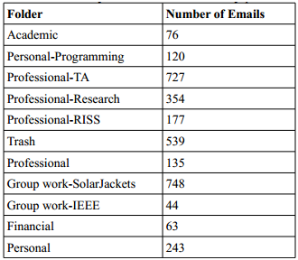
I did this for a bunch of words found in all my emails, and also for the top 20 senders of the emails (since in some cases the sender should correlate strongly with the category, such as the sender being my research adviser and the category ‘research’), and for the top 5 domains the email was sent from (since a few domans like @gatech.edu would be strongly indicative for categories like ‘TA’ and ‘academic’). So, after an hour or so of writing mbox parsing code I ended up with the function that output my actual dataset as a csv.

So, how well did it work? Well, but not as well as I hoped. At the time I was fond of the Orange Python ML framework, and so as per the assignment tested how well a bunch of algorithms did against my dataset. The standouts were decision trees, as the best algorithm, and neural nets, as the worst:

If you take a close look at those beautiful OpenOffice Calc plots, you will see that the best Decision Trees managed to achieve on the test set is roughly 72%, and that neural nets could only get to a measly 65% - an F! Way better than random, considering there are 11 categories, but far from great.

Why the disappointing result? Well, as we saw the features created for the dataset are very simple - just selecting the 500 most frequent words will yield a few good indicators, but also many generic terms that just appear a lot in english such as ‘that’ or ‘is’. I understood this at the time and tried a few things - removing 3-character words entirely, and writing some annoying code to select the most frequent words in each category specifically rather than in all the emails - but ultimately did not manage to figure out how to get better results.

If At First You Don’t Succeed…

So, why am I writing this, if I did this years ago and got fairly lame results (albeit a good grade) then? In short, to try again. With a couple more years of experience, and having just completed a giant 4-part history of neural networks and Deep Learning, it seemed only appropriate to dive into a modern machine learning framework and see what I could do.

But, where to start? By picking the tools, of course! The framework I decided to try is Keras, both because it is in Python (which seems to be a favorite for data science and machine learning nowdays, and plays nice with the wonderful numpy, pandas, and scikit-learn) and because it is backed by the well regarded Theano library.

It also just so happens that Keras has several easy to copy-paste examples to get started with, including one with a multi-category text classification problem. And, here’s the interesting thing - the example uses just about the same features as I did for my class project. It finds the 1000 most frequent words in the documents, makes those into binary features, and trains a neural net with one hidden layer and dropout to predict the category of input text based solely of those features.

So, the obvious first thing to try is exactly this, but with my own data - see if doing feature extraction with Keras will work better. Luckily, I can still use my old mbox parsing code, and Keras has a handy Tokenizer class for text feature extraction. So, it is easy to create a dataset in the same format as in the Keras example, and get an update on my current email counts while we’re at it:

Using Theano backend.
Label email count breakdown:
	Personal:440
	Group work:150
	Financial:118
	Academic:1088
	Professional:388
	Group work/SolarJackets:1535
	Personal/Programming:229
	Professional/Research:1066
	Professional/TA:1801
	Sent:513
	Unread:146
	Professional/EPFL:234
	Important:142
	Professional/RISS:173
Total emails: 8023

Eight thousand emails - not a giant dataset by any stretch, but nevertheless enough to do some serious machine learning. Having converted the data to the correct format, now it is just a matter of seeing if training a neural net with it works. The Keras example makes it very easy to go ahead and do just that:

7221 train sequences
802 test sequences
Building model...
Train on 6498 samples, validate on 723 samples
Epoch 1/5
6498/6498 [==============================] - 2s - loss: 1.3182 - acc: 0.6320 - val_loss: 0.8166 - val_acc: 0.7718
Epoch 2/5
6498/6498 [==============================] - 2s - loss: 0.6201 - acc: 0.8316 - val_loss: 0.6598 - val_acc: 0.8285
Epoch 3/5
6498/6498 [==============================] - 2s - loss: 0.4102 - acc: 0.8883 - val_loss: 0.6214 - val_acc: 0.8216
Epoch 4/5
6498/6498 [==============================] - 2s - loss: 0.2960 - acc: 0.9214 - val_loss: 0.6178 - val_acc: 0.8202
Epoch 5/5
6498/6498 [==============================] - 2s - loss: 0.2294 - acc: 0.9372 - val_loss: 0.6031 - val_acc: 0.8326
802/802 [==============================] - 0s     
Test score: 0.585222780162

Test accuracy: 0.847880299252

Hell yeah 85% test accuracy! That handily beats the measly 65% score of my old neural net. Awesome.

Except… why?

I mean, my old code was doing basically this - finding the most frequent words, creating a binary matrix of features, and training a neural net with one hidden layer to be the classifier. Perhaps, it is because of this fancy new ‘relu’ neuron, and dropout, and using a non-sgd optimizer? Let’s find out! Since my old features were indeed binary and in a matrix, it takes very little work to make those be the dataset this neural net is trained with. And so, the results:

Epoch 1/5
6546/6546 [==============================] - 1s - loss: 1.8417 - acc: 0.4551 - val_loss: 1.4071 - val_acc: 0.5659
Epoch 2/5
6546/6546 [==============================] - 1s - loss: 1.2317 - acc: 0.6150 - val_loss: 1.1837 - val_acc: 0.6291
Epoch 3/5
6546/6546 [==============================] - 1s - loss: 1.0417 - acc: 0.6661 - val_loss: 1.1216 - val_acc: 0.6360
Epoch 4/5
6546/6546 [==============================] - 1s - loss: 0.9372 - acc: 0.6968 - val_loss: 1.0689 - val_acc: 0.6635
Epoch 5/5
6546/6546 [==============================] - 2s - loss: 0.8547 - acc: 0.7215 - val_loss: 1.0564 - val_acc: 0.6690
808/808 [==============================] - 0s     
Test score: 1.03195088158

Test accuracy: 0.64603960396

Ouch. So yes, my old email-categorizing solution was fairly flawed. I can’t say for sure, but I think it is a mix of overconstraining the features (forcing the top senders, domains, and words from each category to be there) and having too few words. The Keras example just throws the top 1000 words into a big matrix without any more intelligent filtering, and lets the neural net have at it. Not limiting what the features can be lets better ones be discovered, and so the overall accuracy is better.

Well, that, or my code just sucks and has mistakes in it - modifying it to be less restrictive still only nets a 70% accuracy. In any case, it’s clear that I was able to beat my old result by leveraging a newer ML library, so the question now clearly is - can I do better?

Deep Learning Is No Good Here

When I first started looking at the Keras code, I was briefly excited by the mistaken notion that it would use the actual sequence of text, with the words in their original order. It turned out that this was not the case, but that does not mean that it can’t be. Indeed, a very cool recent phenomena in machine learning is the resurgence of recurrent neural nets, which are well suited for dealing with long sequences of data. Additionally, when dealing with words it is common to perform an ‘embedding’ step in which each word is converted into a vector of numbers, so that similar words are converted into similar vectors.

So, instead of changing the emails into matrices of binary features it’s possible to just change the words into numbers using the words’ frequency ranking, and the numbers themselves will be converted into vectors which represent the ‘idea’ of each word. Then, we can use the sequence to train a recurrent neural net with Long Short Term Memory or Gated Recurrent units to do the classification. And, guess what? There is also a nice Keras example that does just this, so it is easy to fire up and see what happens:

Epoch 1/15
7264/7264 [===========================] - 1330s - loss: 2.3454 - acc: 0.2411 - val_loss: 2.0348 - val_acc: 0.3594
Epoch 2/15
7264/7264 [===========================] - 1333s - loss: 1.9242 - acc: 0.4062 - val_loss: 1.5605 - val_acc: 0.5502
Epoch 3/15
7264/7264 [===========================] - 1337s - loss: 1.3903 - acc: 0.6039 - val_loss: 1.1995 - val_acc: 0.6568
...
Epoch 14/15
7264/7264 [===========================] - 1350s - loss: 0.3547 - acc: 0.9031 - val_loss: 0.8497 - val_acc: 0.7980
Epoch 15/15
7264/7264 [===========================] - 1352s - loss: 0.3190 - acc: 0.9126 - val_loss: 0.8617 - val_acc: 0.7869
Test score: 0.861739277323

Test accuracy: 0.786864931846

Darn it. Not only did the LSTM take FOREVER, but the results at the end were not that good. Presumably the reason for this is that my emails are just not that much data, and in general sequences are not that useful for categorizing them. That is, the added complexity of learning on sequences does not overcome the benefit of seeing the text in the correct order, since the sender and individual words in the email are good indicators of which category the email should be in as it is.

But, the extra embedding step still seems like it should be useful, since it creates a richer representation of the word. So it seems worthwhile to still try to use it, and also include the important Deep Learning tool of convolution on the text to find important local features. Once again, there is a Keras example that still does embedding but feeds those vector into convolution and pooling layers instead of LSTM layers. But, the results once again are not that impressive:

Epoch 1/3
5849/5849 [===========================] - 127s - loss: 1.3299 - acc: 0.5403 - val_loss: 0.8268 - val_acc: 0.7492
Epoch 2/3
5849/5849 [===========================] - 127s - loss: 0.4977 - acc: 0.8470 - val_loss: 0.6076 - val_acc: 0.8415
Epoch 3/3
5849/5849 [===========================] - 127s - loss: 0.1520 - acc: 0.9571 - val_loss: 0.6473 - val_acc: 0.8554
Test score: 0.556200767488

Test accuracy: 0.858725761773

I really hoped learning with sequences and embeddings could be better learning with basic n-gram features, since in theory the former contains more information about the original emails. But, the folk knowledge that Deep Learning is not very useful for small datasets appears to be true here.

It’s The Features, Dummy

Well, hmm, that did not get me that coveted 90% test accuracy… Time to try being a little smarter about this. See, the current approach of making features out of the top 2500 frequent words is rather silly, in that it includes common english words such as ‘i’ or ‘that’ along with useful category specific words such as ‘homework’ or ‘due’. But, it’s tricky to just guess a cutoff of most frequent words, or blacklist some number of words - you never know what turns out to be useful for features, since it is possible I happen to use one plain word more in one category than the others (such as the category ‘Personal’).

So, let’s avoid the guesswork and instead rely on good ol’ feature selection to pick out features that are actually good and filter out silly ones like ‘i’. As with baseline testing, this is easy using scikit and its SelectKBest class, and is fast enough that it barely takes any time compared to running the neural net. So, does this work?

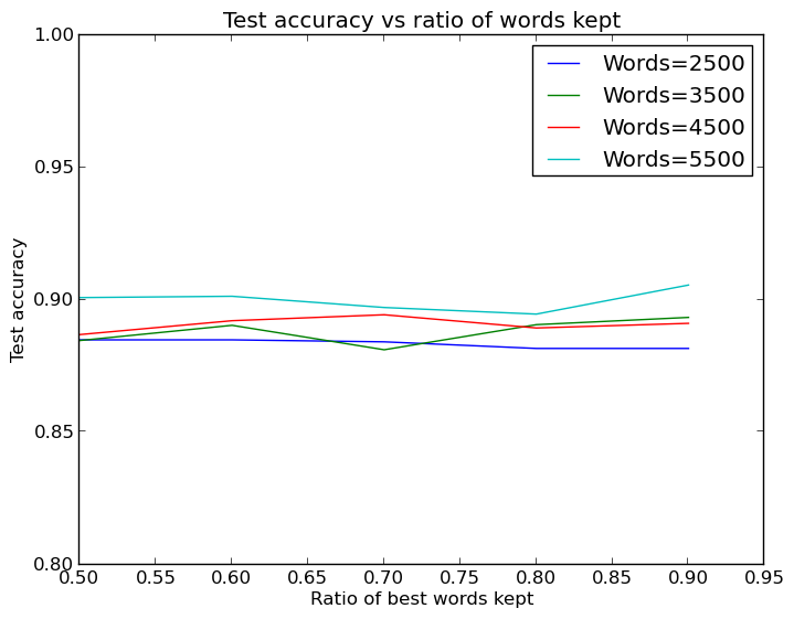
Very nice! Though there is still variance in the performance, more words to start with is clearly better, but this set of words can be cut down rather heavily with feature selection without reducing performance. Apparently the neural net has no problem with undefitting if all the words are kept around. Inspecting the best and worst features according to the feature selector confirms it selects sensible seeming words as good and bad:

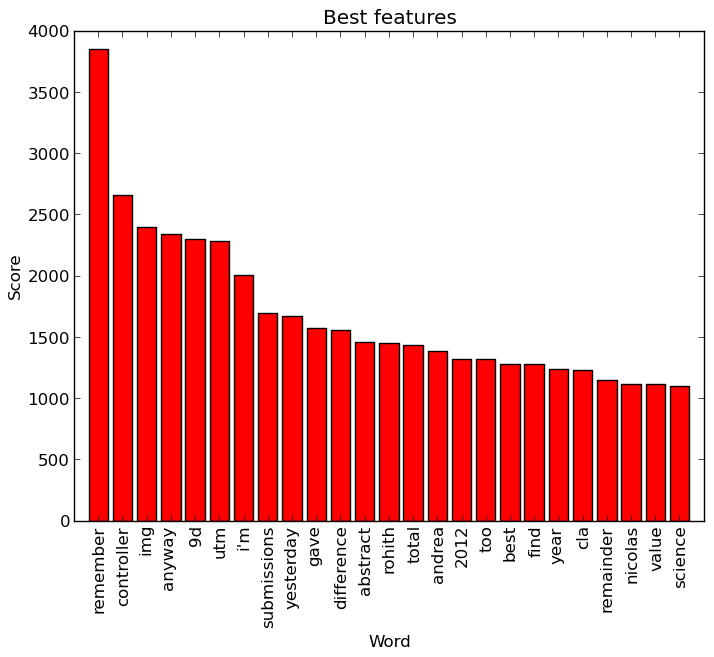
A lot of the best ones are names or refer to specific things (the ‘controller’ is from ‘motor controller’), as could be expected, though a few such as ‘remember’ or ‘total’ would not strike me as very good features. The worst ones, on the other hand, are fairly predictable being either overly generic or overly specific words.

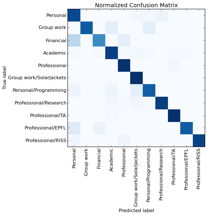
So, the end conclusion is that more words=better, and feature selection can help out by keeping the runtime lower. Well, this helps, but perhaps there is something else to be done to improve performance. To see what, we can look at is what mistakes the neural net makes, with a confusion matrix again from scikit learn:

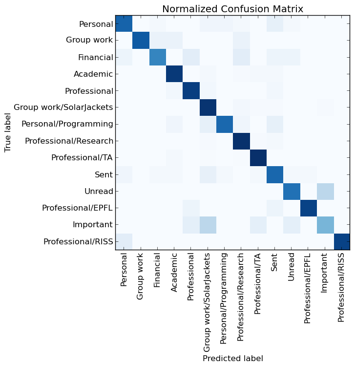
Okay, nice, most of the color is along the diagonal, but there are still some annoying blotches elsewhere. In particular, the visualization implies the ‘Unread’ and ‘Important’ categories are problem makers. But wait! I did not even create those, I don’t really care about things working correctly with them, nor with ‘Sent’. Clearly I should take those out and see if the neural net can do a good job specifically with the categories I created for myself.

So, let’s wrap up with a final experiment in which those irrelevant categories are removed and we use the most features of any run so far - 10000 words with selection of the 4000 best:

Epoch 1/5
5850/5850 [==============================] - 2s - loss: 0.8013 - acc: 0.7879 - val_loss: 0.2976 - val_acc: 0.9369
Epoch 2/5
5850/5850 [==============================] - 1s - loss: 0.1953 - acc: 0.9557 - val_loss: 0.2322 - val_acc: 0.9508
Epoch 3/5
5850/5850 [==============================] - 1s - loss: 0.0988 - acc: 0.9795 - val_loss: 0.2418 - val_acc: 0.9338
Epoch 4/5
5850/5850 [==============================] - 1s - loss: 0.0609 - acc: 0.9865 - val_loss: 0.2275 - val_acc: 0.9462
Epoch 5/5
5850/5850 [==============================] - 1s - loss: 0.0406 - acc: 0.9925 - val_loss: 0.2326 - val_acc: 0.9462
722/722 [==============================] - 0s     
Test score: 0.243211859068

Test accuracy: 0.940443213296

How about that! The neural net can predict categories with 94% accuracy. Though, most of that is due to the large feature set - a good comparison classifier (scikit-learn’s Passive Aggressive classifier) itself gets 91% on the same exact data. In fact following someone else’s suggestion to train a Support Vector Machine classifier (scikits LinearSVC) in a particular way also resulted in roughtly 94% accuracy.

So, the conclusion is fairly straighforward - the fancier methods of Deep Learning do not seem that useful for a small dataset such as my emails, and older approaches such as n-grams + tfifd + SVM can work as well as the most moden neural nets. More generally, just working with a Bag of Words approach works rather well if the data is as small and neatly categorized as this.

I don’t know if few people use categories in gmail, but if it really is this easy to make a classifier that is right most of the time, I would really like it if gmail indeed had such a machine-learned approach to suggesting a category for each email for one-click email organizing. But, for now, I can just feel nice knowing I managed to get a 20% improvement over my last attempt at this, and played with Keras while I was at it.

Epilogue: Extra Experiments

I did a bunch of other things while working on this, and some are worth highlighting. A problem I had all this stuff took forever to run, in large part because I have yet to make use of the now standard trick of doing machine learning with a GPU. So, following a very nice tutorial I did just that, and got nice results:

It should be noted that the Keras neural net with 94% was significantly faster to train and use than the SVM, so it was still ultimately the best approach I have found so far.

I also wanted to do more visualizations besides confusion matrices. There was not much I could with Keras for this, though I did find an ongoing discussion concerning visualization. That led me to a fork of Keras with at least a nice way to graph the training progress. Not very useful, but fun. After hacking it a bit to plot batches instead of epochs, it generated very nice training graphs:

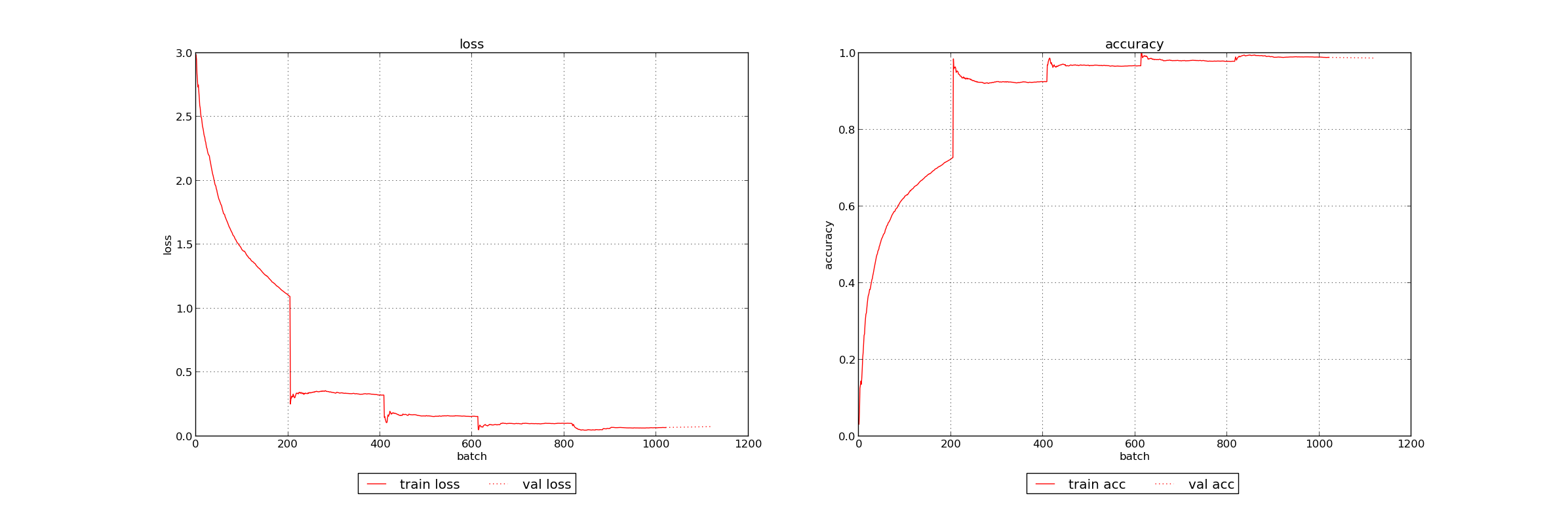
Interesting - the cross validation between epochs results in big jumps in training accuracy, not something I’d expect. But, more pertinently, it’s easy to see the training accuracy just about reaches 1.0 and definitely plateaus.

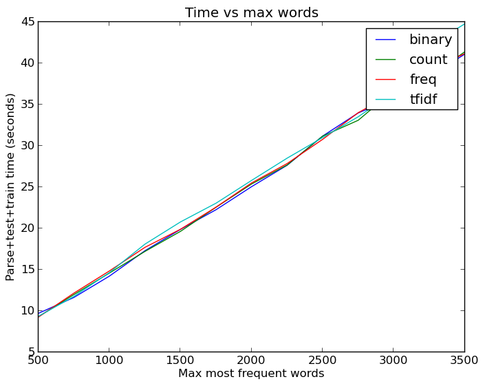
Okay, good, but the harder problem was increasing the test accuracy. As before, the first question is whether I can quickly alter the feature representation to help the neural net out. The Keras module that converts the text into matrices has several options besides making a binary matrix: matrices with word counts, frequencies, or tfidf values. It is also very easy to alter the amount of words kept in the matrices as features, and so being the amazing programmer that I am I managed to write a few loops to evaluate how varying the feature type and word count affects the test accuracy. Not only that, but I even made a pretty plot of the results with python:

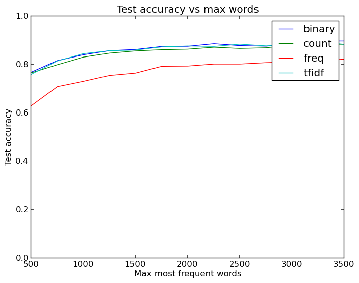
This is where I first saw that I should definitely increase the maximum words to more than 1000. It was also interesting to see that the most basic and least information dense feature type, binary 1s or 0s indicating word presence, is about as good or better than the other features that convey more about the original data. This is not too unexpected, though - most likely more interesting words like ‘code’ or ‘grade’ are helpful for categorization, and having a single occurance in an email is likely almost as informative as more than one. No doubt the more exact features help somewhat, but also lead to worse performance due to more potential for overfitting.

All in all, what we see is that the binary feature type is clearly the best one, and that increasing the number of words helps out quite a bit to get accuracies of about 87%-88%.

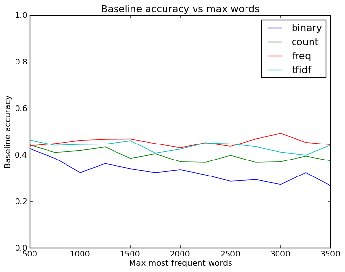
I also looked at baseline algorithms while working on this, to ensure something simple like k nearest neighbors (from scikit) was not equivalent to neural nets, which indeed proved to be true. Linear regression performed even worse, so it seems my use of neural nets is justified.

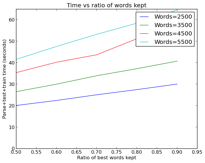
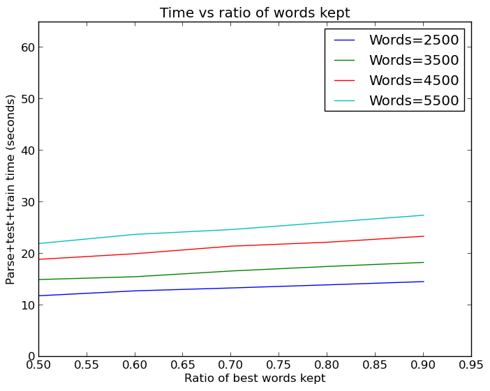
By the way, all this word increasing is not cheap. Even with cached versions of the dataset such that I did not have to parse the emails and extract features each time, running all these tests took a hefty amount of time:

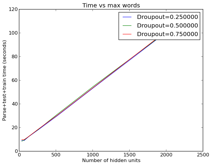
So, increasing the number of words helped, but I was still not cracking the 90% mark - the coveted A threshold! So the next logical thing was to stick with 2500 words and look at varying the neural net size. Also, the example Keras model happened to have 50% dropout on the hidden layer and it was interesting to see if this actually meaningfully helps the performance. So, time to spin up another set of loops and get another pretty graph:

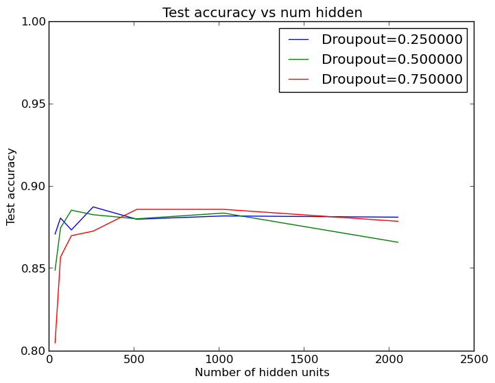
Well, this is somewhat surprising - we don’t need very many hidden layer units at all to do well! With lower dropout (less regularization), as few as 64 and 124 hidden layer units can do just about as well as the default of 512. These results are averaged across five runs, by the way, so mere variation in the outcomes does not account for the ability of small hidden layers to do well. This suggests that the large word counts are good for just including the helpful features, but that there are not really that many helpful features to pick up on - otherwise more neurons would be necessary to do better. This is good to know, since we can save quite a bit of time by using the smaller hidden layers:

But, this is not entirely accurate. More runs with large number of features show that the default hidden layer size of 512 does perform significantly better than a much smaller hidden layer:

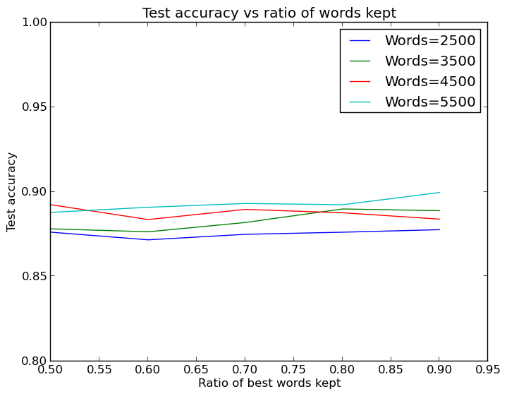
So, in the end we find what we already knew - more words=better.